Predicting car prices with scikit-learn
In this notebook I will attempt to predict automobile prices using Python and its data analysis and machine learning packages such as pandas and scikit-learn. Forecasting car prices can be useful for businesses in general: insurance companies can use this information to calculate their premia; websites and enterprises can provide estimates even when asking prices are not available in a specific application; enterprises can set contracts where a car’s resale value must be defined a priori with greater information, or determine if a car is overvalued or undervalued with respect to the market.
My data source is Mercado Livre, a widely used e-commerce platform in Brazil. For simplicity, and also to isolate other geographical factors that affect prices, this research restricts to ads in the city of Porto Alegre/RS. I also excluded trucks and minivans from the analysis. While new cars can be announced, most of the cars advertised are used. To publish an ad, the seller must fill information about the car, such as brand, model, mileage, engine power and additional features. It is a common belief that this features can help predict a car’s asking price in the market, and in our methodology I will explore them to improve our predictions (of course, there also will be unobservable factors that affect prices). A popular source for automobile prices in Brazil is the FIPE table. In the table, average prices are calculated from newspaper and web ads. Data from the FIPE table can be improved here, as learning models can benefit from data updates, predict prices for cars with a specific set of features and location.
Along the notebook, I will go through all steps of data analysis, with code and commentary.
Data wrangling
First, let’s import the required packages for this step:
import pandas as pd
import matplotlib.pyplot as plt
import seaborn as sns
sns.set()

import numpy as np
import json
import requests
To access data on ads, I’ll make requests to the MercadoLivre’s API. We must build the query URL, using category and location identifiers that can be found in the API documentation site.
# parameters
category = 'MLB1744' # cars and trucks
city     = 'TUxCUFJJT0xkYzM0' # state of rs
limit    = '50'
offset   = [str(i) for i in list(range(50,10000,50))]

# access token
with open('ml_token.txt') as file:
    token = file.read()

#url = 'https://api.mercadolibre.com/sites/MLB/search?category='+category+'&city='+city+'&limit='+limit+'&offset='+offset+'&access_token='+token
Users are only allowed to fetch 50 items per request - up to 10000 items - and this is controlled by the offset parameter. Using requests, we can download all data:
responses = []
for off in offset:
    url = 'https://api.mercadolibre.com/sites/MLB/search?category='+category+'&state='+city+'&limit='+limit+'&offset='+off+'&access_token='+token
    responses.append(requests.get(url))

respd = [i.json() for i in responses]
The .json method transforms the data into a Python dictionary. Looking at the structure of data, I find that ad entries are stored under key results:
respd[0].keys()
dict_keys(['site_id', 'paging', 'results', 'secondary_results', 'related_results', 'sort', 'available_sorts', 'filters', 'available_filters'])
# tests
data1 = [pd.io.json.json_normalize(i['results'], sep='_') for i in respd]
The result is a list of pandas DataFrames. We can append all datasets using concat:
data1 = pd.concat(data1, sort=False).reset_index(drop=True)
data1.head()
| accepts_mercadopago | address_area_code | address_city_id | address_city_name | address_phone1 | address_state_id | address_state_name | attributes | available_quantity | buying_mode | ... | shipping_logistic_type | shipping_mode | shipping_store_pick_up | shipping_tags | site_id | sold_quantity | stop_time | tags | thumbnail | title | |
|---|---|---|---|---|---|---|---|---|---|---|---|---|---|---|---|---|---|---|---|---|---|
| 0 | True | TUxCQ0NBTjcxNTM | Canoas | TUxCUFJJT0xkYzM0 | Rio Grande Do Sul | [{'value_id': '2230581', 'value_name': 'Usado'... | 1 | classified | ... | None | not_specified | False | [] | MLB | 0 | 2019-02-24T04:00:00.000Z | [poor_quality_thumbnail, poor_quality_picture,... | http://mlb-s1-p.mlstatic.com/757910-MLB2918517... | Hyundai Hb20s 1.6 Comfort Plus 16v Flex 4p Manual | ||
| 1 | True | TUxCQ0VOQzZhYTdi | Encantado | TUxCUFJJT0xkYzM0 | Rio Grande Do Sul | [{'value_id': '2230581', 'value_name': 'Usado'... | 1 | classified | ... | None | not_specified | False | [] | MLB | 0 | 2019-02-21T22:16:47.000Z | [poor_quality_picture, poor_quality_thumbnail,... | http://mlb-s1-p.mlstatic.com/671101-MLB2907376... | Chevrolet Agile Ltz - Fernando Multimarcas | ||
| 2 | True | TUxCQ1BPUjgwZTJl | Porto Alegre | TUxCUFJJT0xkYzM0 | Rio Grande Do Sul | [{'source': 1, 'id': 'ITEM_CONDITION', 'name':... | 1 | classified | ... | None | not_specified | False | [] | MLB | 0 | 2019-02-09T09:34:55.000Z | [good_quality_picture, good_quality_thumbnail,... | http://mlb-s2-p.mlstatic.com/962446-MLB2896708... | Renault Grand Scenic 2002 | ||
| 3 | True | TUxCQ0NBWDgxMzcw | Caxias do Sul | TUxCUFJJT0xkYzM0 | Rio Grande Do Sul | [{'id': 'ITEM_CONDITION', 'name': 'Condição do... | 1 | classified | ... | None | not_specified | False | [] | MLB | 0 | 2019-03-19T04:00:00.000Z | [only_html_description, immediate_payment] | http://mlb-s2-p.mlstatic.com/668212-MLB2919195... | Hb20 1.6 Comfort Plus 16v Flex 4p | ||
| 4 | True | TUxCQ1BPUjgwZTJl | Porto Alegre | TUxCUFJJT0xkYzM0 | Rio Grande Do Sul | [{'value_name': 'Automática', 'value_struct': ... | 1 | classified | ... | None | not_specified | False | [] | MLB | 0 | 2019-02-16T04:00:00.000Z | [dragged_visits, good_quality_picture, good_qu... | http://mlb-s1-p.mlstatic.com/968792-MLB2777645... | Volvo Xc90 2.0 T6 Inscription Drive-e 5p |
5 rows × 73 columns
In each entry, we have a series of characteristics on the car, such as make, model, asking price, features and location. Next, I will transform the data into a pandas DataFrame for further manipulation. This requires a few steps, as the data is structured in a list of dicts:
cols = ['title','price','address_city_name','attributes', 'id',
       'location_latitude', 'location_longitude',
       'permalink',
       'seller_car_dealer']

data1 = data1.loc[:,cols]
data1.head()
| title | price | address_city_name | attributes | id | location_latitude | location_longitude | permalink | seller_car_dealer | |
|---|---|---|---|---|---|---|---|---|---|
| 0 | Hyundai Hb20s 1.6 Comfort Plus 16v Flex 4p Manual | 46990.0 | Canoas | [{'value_id': '2230581', 'value_name': 'Usado'... | MLB1167035642 | -29.9188 | -51.1585 | https://carro.mercadolivre.com.br/MLB-11670356... | True |
| 1 | Chevrolet Agile Ltz - Fernando Multimarcas | 28800.0 | Encantado | [{'value_id': '2230581', 'value_name': 'Usado'... | MLB1159937620 | -29.2249 | -51.8895 | https://carro.mercadolivre.com.br/MLB-11599376... | True |
| 2 | Renault Grand Scenic 2002 | 8500.0 | Porto Alegre | [{'source': 1, 'id': 'ITEM_CONDITION', 'name':... | MLB1152825359 | -30.0346 | -51.2177 | https://carro.mercadolivre.com.br/MLB-11528253... | False |
| 3 | Hb20 1.6 Comfort Plus 16v Flex 4p | 44890.0 | Caxias do Sul | [{'id': 'ITEM_CONDITION', 'name': 'Condição do... | MLB1167546961 | -29.1634 | -51.1797 | https://carro.mercadolivre.com.br/MLB-11675469... | True |
| 4 | Volvo Xc90 2.0 T6 Inscription Drive-e 5p | 339950.0 | Porto Alegre | [{'value_name': 'Automática', 'value_struct': ... | MLB1165970712 | -30.0554 | -51.2224 | https://carro.mercadolivre.com.br/MLB-11659707... | True |
It’s a great step forward, however information on a car’s attributes are still trapped in a list of dicts. Hence any attempts at using the previous json_serialize method will fail. As an example, let’s apply the function to the feature alone:
pd.io.json.json_normalize(data1.attributes[0], sep='_').head()
Now, I will reshape the data in order to have a single row per advertising. Let’s define a helper function:
def reshape_(data):
    return data.loc[:,['id','value_name']].set_index('id').transpose()
We must now loop over samples and then join all data. For loops can be avoided, using Python’s list comprehensions:
df_temp = [reshape_(pd.io.json.json_normalize(i)) for i in data1.attributes]

data2 = pd.concat(df_temp, sort=False).reset_index(drop=True)
del df_temp
data2.tail()
| ITEM_CONDITION | TRANSMISSION | ENGINE_DISPLACEMENT | BRAND | DOORS | FUEL_TYPE | KILOMETERS | MODEL | TRIM | VEHICLE_YEAR | TRACTION_CONTROL | |
|---|---|---|---|---|---|---|---|---|---|---|---|
| 9943 | Usado | Manual | 999 cc | Volkswagen | 5 | Gasolina e álcool | 100000 km | Fox | 1.0 Vht Trend Total Flex 5p | 2009 | Dianteira |
| 9944 | Usado | Manual | 999 cc | Ford | 5 | Gasolina | 130000 km | Fiesta | 1.0 Street 5p | 2004 | Dianteira |
| 9945 | Usado | Manual | 1360 cc | Peugeot | 5 | Gasolina e álcool | 124 km | 206 | 1.4 Presence Flex 5p | 2008 | Dianteira |
| 9946 | Usado | Manual | 999 cc | Fiat | 5 | Gasolina e álcool | 95800 km | Palio | 1.0 Fire Celebration Flex 5p | 2009 | Dianteira |
| 9947 | Usado | Manual | 1598 cc | Ford | 5 | Gasolina | 190000 km | Focus | 1.6 Gl 5p | 2007 | Dianteira |
Finally, we’ll merge with the original data:
df = pd.concat([data1,data2], axis=1)
df.head()
| price | address_city_name | location_latitude | location_longitude | seller_car_dealer | transmission | engine_displacement | brand | doors | fuel_type | kilometers | model | vehicle_year | traction_control | |
|---|---|---|---|---|---|---|---|---|---|---|---|---|---|---|
| 0 | 46990.0 | Canoas | -29.918818 | -51.158540 | True | Manual | 1591.0 | hyundai | 4.0 | Gasolina e álcool | 72.258 | hb20s | 2017.0 | Dianteira |
| 1 | 28800.0 | Encantado | -29.224850 | -51.889533 | True | Manual | 1389.0 | chevrolet | 4.0 | Gasolina e álcool | 74.000 | agile | 2011.0 | Dianteira |
| 3 | 44890.0 | Caxias do Sul | -29.163403 | -51.179668 | True | Manual | 1591.0 | hyundai | 4.0 | Gasolina e álcool | 39.293 | hb20 | 2018.0 | Dianteira |
| 5 | 52900.0 | Santa Maria | -29.696541 | -53.799310 | True | Automática | 1598.0 | volkswagen | 4.0 | Gasolina e álcool | 30.600 | crossfox | 2015.0 | 4x2 |
| 6 | 61900.0 | Santa Maria | -29.696541 | -53.799310 | True | Automática | 999.0 | ford | 5.0 | Gasolina | 9.345 | fiesta | 2017.0 | 4x2 |
Some more data cleaning, to deal with strings and data types:
df.drop(['TRIM','ITEM_CONDITION','title','attributes','id','permalink'], axis=1, inplace=True)
df.columns = map(str.lower, df.columns)

#remove unwanted strings
cols = ['location_latitude', 'location_longitude','engine_displacement','kilometers','vehicle_year','doors']
df.loc[:,cols] = df.loc[:,cols].replace(regex=True,to_replace=r'\D',value=r'')

# replace empty strings with NaN
df.replace({'':np.nan}, inplace=True)

# set brand and model strings to lowercase
df.brand = df.brand.str.lower()
df.model = df.model.str.lower()
# type conversion
df = df.astype({'location_latitude':float, 'location_longitude':float,'engine_displacement':float,
                'kilometers':float,'vehicle_year':float,'doors':float})

df.dtypes
price                  float64
address_city_name       object
location_latitude      float64
location_longitude     float64
seller_car_dealer         bool
transmission            object
engine_displacement    float64
brand                   object
doors                  float64
fuel_type               object
kilometers             float64
model                   object
vehicle_year           float64
traction_control        object
dtype: object
Now, I will attempt to detect outliers in numerical features. We must note that some extreme values are not outliers (i.e. we will have feature kilometers set to zero for new cars). Outlier detection will generate missing values that must be treated later.
df.describe().round(2)
| price | location_latitude | location_longitude | engine_displacement | doors | kilometers | vehicle_year | |
|---|---|---|---|---|---|---|---|
| count | 9740.00 | 9740.00 | 9740.00 | 9740.00 | 9740.00 | 9740.00 | 9740.00 |
| mean | 47753.99 | -29.70 | -51.29 | 1653.57 | 3.97 | 57.63 | 2012.58 |
| std | 32267.50 | 1.17 | 0.99 | 528.68 | 0.76 | 51.19 | 4.39 |
| min | 8999.00 | -33.69 | -57.55 | 994.00 | 0.00 | 0.00 | 1960.00 |
| 25% | 27900.00 | -30.02 | -51.20 | 1368.00 | 4.00 | 21.00 | 2011.00 |
| 50% | 37900.00 | -29.95 | -51.18 | 1598.00 | 4.00 | 54.00 | 2013.00 |
| 75% | 56040.00 | -29.70 | -51.14 | 1975.00 | 4.00 | 83.00 | 2015.00 |
| max | 249000.00 | -6.93 | -37.88 | 3960.00 | 7.00 | 920.00 | 2019.00 |
# fix extreme values
df.price.replace({df.price.max(): np.nan}, inplace=True)
df.engine_displacement[df.engine_displacement < 900] = np.nan
df.engine_displacement[df.engine_displacement > 4000] = np.nan
df.kilometers.replace({df.kilometers.max(): np.nan}, inplace=True)
df.vehicle_year.replace({df.vehicle_year.min(): np.nan}, inplace=True)
Finally, we must deal with missing values, since scikit-learn does not accept them. It is often more fruitful to fill in missing values, rather than dropping whole samples.
# find missing values
df.isna().sum()
price                  0
address_city_name      0
location_latitude      0
location_longitude     0
seller_car_dealer      0
transmission           0
engine_displacement    0
brand                  0
doors                  0
fuel_type              0
kilometers             0
model                  0
vehicle_year           0
traction_control       0
dtype: int64
df.transmission       = df.transmission.fillna('Manual')
df.kilometers         = df.kilometers.fillna(df.kilometers.mean())
df.price              = df.price.fillna(df.price.mean())
df.traction_control   = df.traction_control.fillna('Dianteira')
df.location_latitude  = df.location_latitude.fillna(method='ffill')
df.location_longitude = df.location_longitude.fillna(method='ffill')
df.vehicle_year       = df.vehicle_year.fillna(df.vehicle_year.mean())
Features engine_displacement still exhibit lots of missing values. For engine_displacement, my strategy was to fill with the mode (or median) values of features according to each car model. This seems to be a better approach than filling with the average engine size of all cars.
import statistics
def mode_or_median(var):
    try:
        return statistics.mode(var)
    except statistics.StatisticsError: # there may be no unique value
        return np.median(var)
avg_eng = df.groupby('model')['engine_displacement'].apply(mode_or_median)
avg_eng.fillna(avg_eng.median(),inplace=True) # fill the remaining NaN's
avg_eng.sample(10)
Now, we will insert the average values only when data were initially missing:
df.set_index('model', drop=False, inplace=True)
df.update(avg_eng, overwrite=False) # overwrite=False only updates NaN's
df.reset_index(drop=True, inplace=True)
Last, I will drop extreme values from our target distribution of car prices. First, because luxury car prices are harder to predict (because of fewer data points), and also because some entries are just wrong (i.e. ads for older cars whose prices have been mistyped).
# keep values within interval
df = df[(df.price > df.price.quantile(0.01)) & (df.price < df.price.quantile(0.99))]
Finally, we have a dataset ready for analysis:
df.head()
| price | address_city_name | location_latitude | location_longitude | seller_car_dealer | transmission | engine_displacement | brand | doors | fuel_type | kilometers | model | vehicle_year | traction_control | |
|---|---|---|---|---|---|---|---|---|---|---|---|---|---|---|
| 0 | 46990.0 | Canoas | -29.918818 | -51.158540 | True | Manual | 1591.0 | hyundai | 4.0 | Gasolina e álcool | 72.258 | hb20s | 2017.0 | Dianteira |
| 1 | 28800.0 | Encantado | -29.224850 | -51.889533 | True | Manual | 1389.0 | chevrolet | 4.0 | Gasolina e álcool | 74.000 | agile | 2011.0 | Dianteira |
| 3 | 44890.0 | Caxias do Sul | -29.163403 | -51.179668 | True | Manual | 1591.0 | hyundai | 4.0 | Gasolina e álcool | 39.293 | hb20 | 2018.0 | Dianteira |
| 5 | 52900.0 | Santa Maria | -29.696541 | -53.799310 | True | Automática | 1598.0 | volkswagen | 4.0 | Gasolina e álcool | 30.600 | crossfox | 2015.0 | 4x2 |
| 6 | 61900.0 | Santa Maria | -29.696541 | -53.799310 | True | Automática | 999.0 | ford | 5.0 | Gasolina | 9.345 | fiesta | 2017.0 | 4x2 |
Exploratory data analysis
First, let’s check descriptive statistics:
#df.to_csv('~/mlcars.csv', index=False)
df = pd.read_csv('C:/Users/gsalt/mlcars.csv')
df.describe(include='all').round(2)
| price | address_city_name | location_latitude | location_longitude | seller_car_dealer | transmission | engine_displacement | brand | doors | fuel_type | kilometers | model | vehicle_year | traction_control | |
|---|---|---|---|---|---|---|---|---|---|---|---|---|---|---|
| count | 9740.00 | 9740 | 9740.00 | 9740.00 | 9740 | 9740 | 9740.00 | 9740 | 9740.00 | 9740 | 9740.00 | 9740 | 9740.00 | 9740 |
| unique | NaN | 147 | NaN | NaN | 2 | 4 | NaN | 49 | NaN | 12 | NaN | 440 | NaN | 5 |
| top | NaN | Porto Alegre | NaN | NaN | True | Manual | NaN | chevrolet | NaN | Gasolina e álcool | NaN | onix | NaN | Dianteira |
| freq | NaN | 4103 | NaN | NaN | 9019 | 6008 | NaN | 1514 | NaN | 6910 | NaN | 280 | NaN | 7812 |
| mean | 47753.99 | NaN | -29.70 | -51.29 | NaN | NaN | 1653.57 | NaN | 3.97 | NaN | 57.63 | NaN | 2012.58 | NaN |
| std | 32267.50 | NaN | 1.17 | 0.99 | NaN | NaN | 528.68 | NaN | 0.76 | NaN | 51.19 | NaN | 4.39 | NaN |
| min | 8999.00 | NaN | -33.69 | -57.55 | NaN | NaN | 994.00 | NaN | 0.00 | NaN | 0.00 | NaN | 1960.00 | NaN |
| 25% | 27900.00 | NaN | -30.02 | -51.20 | NaN | NaN | 1368.00 | NaN | 4.00 | NaN | 21.00 | NaN | 2011.00 | NaN |
| 50% | 37900.00 | NaN | -29.95 | -51.18 | NaN | NaN | 1598.00 | NaN | 4.00 | NaN | 54.00 | NaN | 2013.00 | NaN |
| 75% | 56040.00 | NaN | -29.70 | -51.14 | NaN | NaN | 1975.00 | NaN | 4.00 | NaN | 83.00 | NaN | 2015.00 | NaN |
| max | 249000.00 | NaN | -6.93 | -37.88 | NaN | NaN | 3960.00 | NaN | 7.00 | NaN | 920.00 | NaN | 2019.00 | NaN |
The describe method is very useful to find strange values left in data, such as found in engine displacement and kilometers.
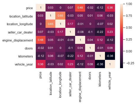
The correlation matrix:
sns.heatmap(df.corr().round(2), annot=True)
<matplotlib.axes._subplots.AxesSubplot at 0x285fae7c208>
The most popular cars announced and the average price:
df.groupby(['brand','model']).agg({'price':['mean','count']}).sort_values(('price','count'), ascending=False)[:10]
| price | |||
|---|---|---|---|
| mean | count | ||
| brand | model | ||
| chevrolet | onix | 40334.564250 | 280 |
| fiat | palio | 25952.777778 | 270 |
| renault | sandero | 32828.739837 | 246 |
| volkswagen | gol | 23750.466667 | 240 |
| ford | fiesta | 32778.090909 | 231 |
| volkswagen | fox | 31756.559633 | 218 |
| fiat | uno | 27420.529126 | 206 |
| ford | ecosport | 48480.684211 | 190 |
| citroën | c3 | 32972.803371 | 178 |
| ford | ka | 32543.722543 | 173 |
The same query as before, now considering the manufacturing year of the cars:
df.groupby(['brand','model','vehicle_year']).agg({'price':['mean','count']}).sort_values(('price','count'), ascending=False)[:10]
| price | ||||
|---|---|---|---|---|
| mean | count | |||
| brand | model | vehicle_year | ||
| fiat | mobi | 2018.0 | 33558.644068 | 59 |
| ford | ka | 2018.0 | 39714.827586 | 58 |
| chevrolet | onix | 2015.0 | 39301.210526 | 57 |
| 2018.0 | 39498.392857 | 56 | ||
| ford | fiesta | 2014.0 | 33070.696429 | 56 |
| jeep | renegade | 2016.0 | 75305.489796 | 49 |
| chevrolet | onix | 2016.0 | 42870.638085 | 47 |
| fiat | uno | 2018.0 | 32799.565217 | 46 |
| chevrolet | onix | 2017.0 | 43780.888889 | 45 |
| renault | sandero | 2018.0 | 37992.222222 | 45 |
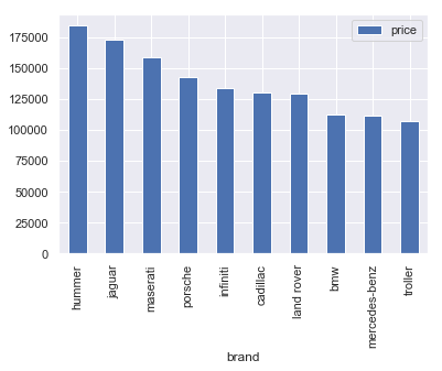
Here are the most expensive brands, by average price:
df.pivot_table(index=['brand'], values=['price'], aggfunc=np.mean).round(2).sort_values('price', ascending=False)[:10].plot.bar()
<matplotlib.axes._subplots.AxesSubplot at 0x285fb184828>
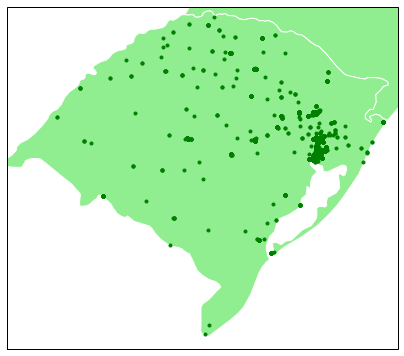
How cars are located geographically:
import cartopy.crs as ccrs
from cartopy.io import shapereader

kw = dict(resolution='50m', category='cultural',
          name='admin_1_states_provinces')

states_shp = shapereader.natural_earth(**kw)
shp = shapereader.Reader(states_shp)

subplot_kw = dict(projection=ccrs.PlateCarree())

fig, ax = plt.subplots(figsize=(7, 11),
                       subplot_kw=subplot_kw)
ax.set_extent([-57.5,-49.5, -34,-27])
ax.add_geometries(shp.geometries(), ccrs.PlateCarree(), facecolor='lightgreen')
ax.scatter(df.location_longitude, df.location_latitude, marker='.', c='green', zorder=2)
<matplotlib.collections.PathCollection at 0x285869b1f98>
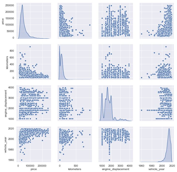
The relationship between continuous features are key in our dataset. Are they linear? This is important as most models assume a linear relationship between features and the target.
sns.pairplot(df[['price','kilometers','engine_displacement','vehicle_year']], diag_kind='kde')
C:\Users\gsalt\Anaconda3\lib\site-packages\scipy\stats\stats.py:1713: FutureWarning: Using a non-tuple sequence for multidimensional indexing is deprecated; use `arr[tuple(seq)]` instead of `arr[seq]`. In the future this will be interpreted as an array index, `arr[np.array(seq)]`, which will result either in an error or a different result.
  return np.add.reduce(sorted[indexer] * weights, axis=axis) / sumval


<seaborn.axisgrid.PairGrid at 0x285885ec6d8>
Model tests
First, let’s identify the scope of our problem. Our target, price, is continuous, so we’re dealing with a regression problem. In this section I will experiment with different regression techniques. But first, the dataset must be further processed: our categorical features must be translated into numeric. This can be done in pandas with get_dummies (or in scikit-learn with OneHotEncoder): it transforms a categorical feature into dummy variables that indicate which category an observation belongs.’
My theoretical model is currently specified as (simplified):
\[price_i = model_i + year_i + features_i + error_i\]In a regression context, this means that all auto models depreciate at a rate determined by the coefficient associated with \(year\). However, one would expect each model to lose value at a different rate (i.e. luxury, fuel-efficient or low-maintenance cars would preserve their value for longer). We can implement this by interacting features \(model\) and \(year\), that is, \(price_i = modelyear_i + features_i + error_i\). The downside of this approach is that it may lead to overfitting.
Let’s load the scikit-learn methods:
from sklearn.compose import ColumnTransformer
from sklearn.pipeline import Pipeline, FeatureUnion
from sklearn.preprocessing import StandardScaler, OneHotEncoder, FunctionTransformer
from sklearn.model_selection import train_test_split
from sklearn import metrics

# disable standard scaler data conversion warning
import warnings
from sklearn.exceptions import DataConversionWarning
warnings.filterwarnings(action='ignore', category=DataConversionWarning)

X = df.drop(['price','address_city_name'], axis=1).copy()
y = df.price.values.copy() # prices in R$
Next, I split the data in both training and data sets. Training data will be used to fit the model, and the test set to assess model accuracy.
# generate train and test sets
X_train, X_test, y_train, y_test = train_test_split(X, y, test_size=0.3)
In addition, we can perform standardization (centering of data around the average, also called scaling) of our numerical features using StandardScaler. Standardization can improve the accuracy of most models, on the other hand we lose interpretation of model coefficients such as the ones given by linear regression. Fortunately, we can use the predict method to give us model predictions. This step will be done inside a pipeline, after training and test data splits, to avoid data leakage.
# categorical features
cat_ft = ['seller_car_dealer', 'transmission', 'brand', 'fuel_type', 'model', 'traction_control']

# run once on full dataset to get all category values
temp = ColumnTransformer([('cat', OneHotEncoder(), cat_ft)]).fit(X)
cats = temp.named_transformers_['cat'].categories_

cat_tr = OneHotEncoder(categories=cats, sparse=False)

# numerical features
num_ft = ['location_latitude', 'location_longitude', 'engine_displacement', 'doors', 'kilometers', 'vehicle_year']
num_tr = StandardScaler()
#num_tr = FunctionTransformer(func=None)

# data transformer
data_tr = ColumnTransformer([('num', num_tr, num_ft), ('cat', cat_tr, cat_ft)])
Model comparison
There are a lot of techniques that can be used in a regression problem. As a starting point, I will compare some of them in terms of scores and sum of errors:
from sklearn import linear_model
from sklearn.neighbors import KNeighborsRegressor
from sklearn.dummy import DummyRegressor
from sklearn import ensemble

models = [DummyRegressor(),
          KNeighborsRegressor(),
          #linear_model.LinearRegression(), # ommited because of negative scores
          linear_model.Lasso(),
          linear_model.Ridge(),
          linear_model.ElasticNet(),
          ensemble.GradientBoostingRegressor(),
          ensemble.RandomForestRegressor(),
          ensemble.ExtraTreesRegressor()]

models_names = ['Dummy','K-nn','Lasso','Ridge','Elastic','Boost','Forest','Extra']
scores = []
mse = []
mae = []

for model in models:
    pipe = Pipeline([
    ('features', data_tr),
    ('model', model)
    ])
    fits = pipe.fit(X_train,y_train)
    scores.append(metrics.r2_score(y_test, fits.predict(X_test)))
    mse.append(metrics.mean_squared_error(y_test, fits.predict(X_test)))
    mae.append(metrics.median_absolute_error(y_test, fits.predict(X_test)))
C:\Users\gsalt\Anaconda3\lib\site-packages\sklearn\linear_model\coordinate_descent.py:492: ConvergenceWarning: Objective did not converge. You might want to increase the number of iterations. Fitting data with very small alpha may cause precision problems.
  ConvergenceWarning)
C:\Users\gsalt\Anaconda3\lib\site-packages\sklearn\ensemble\forest.py:246: FutureWarning: The default value of n_estimators will change from 10 in version 0.20 to 100 in 0.22.
  "10 in version 0.20 to 100 in 0.22.", FutureWarning)
C:\Users\gsalt\Anaconda3\lib\site-packages\sklearn\ensemble\forest.py:246: FutureWarning: The default value of n_estimators will change from 10 in version 0.20 to 100 in 0.22.
  "10 in version 0.20 to 100 in 0.22.", FutureWarning)
Let’s take a look at the model \(R^2\) scores (more is better), mean squared error and median absolute error (less is better):
f, (ax1, ax2, ax3) = plt.subplots(ncols=3, sharex=True, sharey=False, figsize=(18,6))
ax1.bar(models_names, scores)
ax1.set_ylabel('$R^2$')
ax2.bar(models_names, mse)
ax2.set_ylabel('Mean squared error')
ax3.bar(models_names, mae)
ax3.set_ylabel('Median absolute error')
Text(0, 0.5, 'Median absolute error')
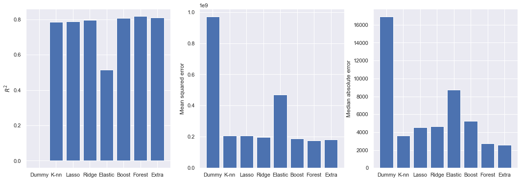
All model scores are calculated using regression residuals, so they are correlated. The \(R^2\) score in most models performed at around 0.8, except the elastic net model, which peaked at 0.5 in the training set. Gradient boosting, random forest and extra trees had the best scores. However, \(R^2\) scores should be taken with precaution as they are biased towards larger models. Mean squared error (MSE) is a metric that penalizes larger prediction errors. Last are the median absolute error (MAE). Absolute error measures are interesting because they inform average deviations in terms of our target (predicted car prices, in our case).
I’ll stick with the random forest regressor, as it was less prone to overfitting in previous tests.
Predictions
Now, we fit the chosen model and extract some predictions:
mod = Pipeline([
    ('features', data_tr),
    ('model', ensemble.RandomForestRegressor(n_estimators=100, min_samples_leaf=1))])

mod_fit = mod.fit(X_train, y_train)

mod_fit.score(X_test,y_test)
Some example predictions from the model:
pred = pd.DataFrame.from_dict({'predicted':mod_fit.predict(X_test), 'true':y_test})
pred['difference'] = pred.predicted - pred.true
pred.sample(n=10).round(2)
| predicted | true | difference | |
|---|---|---|---|
| 2386 | 36963.40 | 34990.0 | 1973.40 |
| 144 | 162293.38 | 150000.0 | 12293.38 |
| 1175 | 31838.20 | 32960.0 | -1121.80 |
| 2155 | 29880.00 | 29900.0 | -20.00 |
| 1052 | 44718.00 | 44500.0 | 218.00 |
| 1759 | 32580.00 | 31900.0 | 680.00 |
| 622 | 27303.20 | 23900.0 | 3403.20 |
| 2363 | 40363.60 | 42900.0 | -2536.40 |
| 429 | 32632.40 | 33900.0 | -1267.60 |
| 2709 | 39779.80 | 33900.0 | 5879.80 |
The average prediction error in car prices is around -R$600. The value being negative means that the model tends to underestimate prices in general. The not-so-good news is that the standard deviation of predictions is pretty high.
pred.difference.describe()
count      2922.000000
mean       -632.707264
std       13053.008512
min     -189274.200000
25%       -2489.150000
50%         150.560000
75%        2949.950000
max       80052.000000
Name: difference, dtype: float64
Model tuning
The random forest regressor have a few hyperparameters that can be tuned to improve overall accuracy. I will play around with n_estimators (the number of estimators/trees) and min_samples_leaf (the minimum number of samples to be in a tree branch). One might be tempted to test all parameters, but the computational costs quickly grow according to the number of parameters, possible values and cross-validation folds:
from sklearn.model_selection import GridSearchCV

# cross validation folds
folds=3

# set parameter range for grid search
params = {'model__n_estimators': [10, 20, 30, 50, 100], 'model__min_samples_leaf': [1,2]}

grids = GridSearchCV(mod, param_grid=params, cv=folds)
grids_fit = grids.fit(X_train, y_train)

print('Best choice of parameter:', grids_fit.best_params_)
Best choice of parameter: {'model__min_samples_leaf': 1, 'model__n_estimators': 100}
Validation
First, I will perform a three-fold cross validation (that is, calculate training and test scores for three random sub-samples of data) and take the mean of scores:
from sklearn.model_selection import cross_validate

mod_cross_val = cross_validate(mod, X, y=y, cv=folds, return_train_score=True)

print('Average train score:', mod_cross_val['train_score'].mean().round(4))
print('Average test score:',  mod_cross_val['test_score'].mean().round(4))
Average train score: 0.9766709555336993
Average test score: 0.8178101080682266
Next, the learning curve tells us how model prediction improves as we add training samples (that’s when the machine is learning):
from sklearn.model_selection import learning_curve

learn_tr_size, learn_train_sc, learn_test_sc = learning_curve(mod, X_train, y_train, cv=folds)

# calculate mean over cross-validation folds
learn_train_m = np.apply_along_axis(np.mean, 1, learn_train_sc)
learn_test_m  = np.apply_along_axis(np.mean, 1, learn_test_sc)

plt.plot(learn_tr_size, learn_train_m)
plt.plot(learn_tr_size, learn_test_m)
plt.title('Learning curve')
plt.xlabel('Training samples')
plt.ylabel('Scores')
plt.legend(['Train score','Test score'])
<matplotlib.legend.Legend at 0x2859d6e8d68>
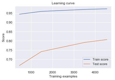
The learning curve tells us that our model performs much better in training than in test data, although both scores improve as we add samples. Intuitively, this means that the model struggles to generalize to new, unknown cases. Improvements can be made in the following senses:
- Model tuning: Results from the learning curve are a sign of overfitting. A solution could be fitting a more parsimonious tree.
- Feature engineering: in a regression context, having a single coefficient for
kilometersmeans that all cars depreciate at a constant rate. But we know that luxury or fuel-efficient models keep their value for longer. A solution would be the creation of features that are interactions ofmodelandvehicle_year.